Text Mining
USING TIDY DATA PRINCIPLES
Hello!

Let’s install some packages
Workflow for text mining/modeling
Topic modeling
📖 Each DOCUMENT = mixture of topics
📑 Each TOPIC = mixture of tokens
Tip
Topic modeling is an example of unsupervised machine learning.
GREAT LIBRARY HEIST 🕵
Download your text data
library(tidyverse)
library(gutenbergr)

books <- gutenberg_download(c(36, 55, 158, 768),
                            meta_fields = "title",
                            mirror = my_mirror)
books |>
    count(title)
#> # A tibble: 4 × 2
#>   title                          n
#>   <chr>                      <int>
#> 1 Emma                       16488
#> 2 The War of the Worlds       6372
#> 3 The Wonderful Wizard of Oz  4750
#> 4 Wuthering Heights          12342
Someone has torn up your books! 😭
What do you predict will happen if we run the following code? 🤔
Someone has torn up your books! 😭
What do you predict will happen if we run the following code? 🤔
books_by_document <- books |>
    group_by(title) |>
    mutate(document = row_number() %/% 500) |>
    ungroup() |>
    unite(document, title, document)

glimpse(books_by_document)
#> Rows: 39,952
#> Columns: 3
#> $ gutenberg_id <int> 36, 36, 36, 36, 36, 36, 36, 36, 36, 36, 36, 36, 36, 36, 3…
#> $ text <chr> "cover ", "", "", "", "", "The War of the Worlds", "", "b…
#> $ document <chr> "The War of the Worlds_0", "The War of the Worlds_0", "Th…Can we put them back together?
library(tidytext)

word_counts <- books_by_document |>
    unnest_tokens(word, text) |>
    anti_join(get_stopwords(source = "smart")) |>
    count(document, word, sort = TRUE)

glimpse(word_counts)
#> Rows: 81,289
#> Columns: 3
#> $ document <chr> "The Wonderful Wizard of Oz_4", "Emma_0", "Emma_7", "Emma_2",…
#> $ word     <chr> "green", "chapter", "mr", "mr", "dorothy", "mr", "mr", "mr", …
#> $ n        <int> 61, 57, 56, 54, 53, 52, 51, 50, 49, 48, 47, 46, 44, 44, 43, 4…
Tip
The dataset word_counts contains the counts of words per line.
Can we put them back together?
Tip
Is words_sparse a tidy dataset?
Train a topic model
Use a sparse matrix or a quanteda::dfm object as input:
Train a topic model
Use a sparse matrix or a quanteda::dfm object as input:
summary(topic_model)
#> A topic model with 4 topics, 81 documents and a 15067 word dictionary.
#> Topic 1 Top Words:
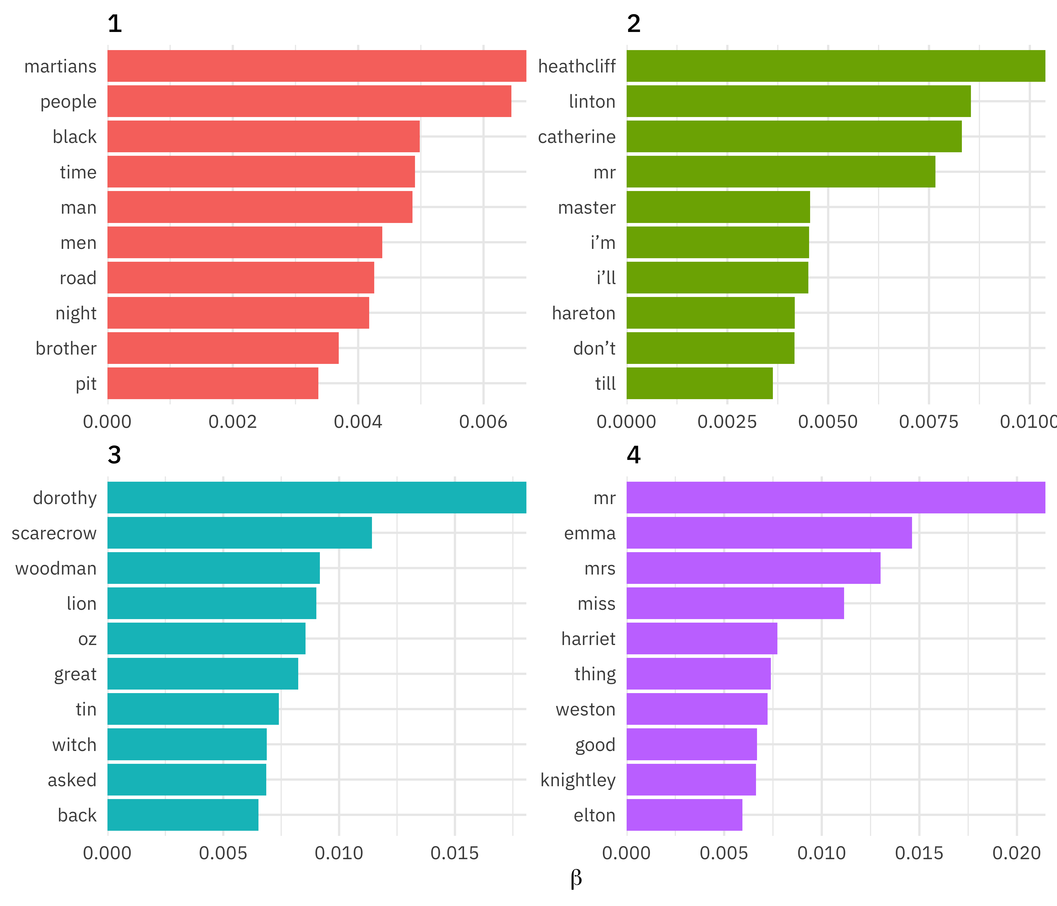
#>       Highest Prob: martians, people, black, time, man, men, road
#>       FREX: martians, martian, smoke, cylinder, woking, machine, mars
#>       Lift: maybury, meteorite, venus, _thunder, child_, ironclads, _daily
#>       Score: martians, martian, cylinder, woking, smoke, machine, mars
#> Topic 2 Top Words:
#>       Highest Prob: heathcliff, linton, catherine, mr, master, i’m, i’ll
#>       FREX: linton, catherine, cathy, edgar, heights, nelly, wuthering
#>       Lift: she’s, dean, catherine’s, crags, moor, drawer, daddy
#>       Score: heathcliff, linton, catherine, hareton, cathy, joseph, earnshaw
#> Topic 3 Top Words:
#>       Highest Prob: dorothy, scarecrow, woodman, lion, oz, great, tin
#>       FREX: dorothy, scarecrow, woodman, lion, oz, witch, toto
#>       Lift: woodman, toto, china, munchkins, winged, glinda, wizard
#>       Score: dorothy, scarecrow, woodman, oz, lion, toto, witch
#> Topic 4 Top Words:
#>       Highest Prob: mr, emma, mrs, miss, harriet, thing, weston
#>       FREX: emma, harriet, weston, knightley, elton, jane, woodhouse
#>       Lift: fairfax, harriet, elton, taylor, elton’s, charade, dixon
#>       Score: emma, harriet, weston, knightley, elton, jane, mr
Explore the topic model output
chapter_topics <- tidy(topic_model, matrix = "beta")
chapter_topics
#> # A tibble: 60,268 × 3
#>    topic term         beta
#>    <int> <chr>       <dbl>
#>  1     1 green   1.70e-  3
#>  2     2 green   2.01e-  4
#>  3     3 green   5.83e-  3
#>  4     4 green   1.55e-160
#>  5     1 chapter 7.99e-  5
#>  6     2 chapter 6.63e-  4
#>  7     3 chapter 2.98e-  3
#>  8     4 chapter 2.07e-  3
#>  9     1 mr      2.28e-102
#> 10     2 mr      7.66e-  3
#> # ℹ 60,258 more rows
Explore the topic model output
U N S C R A M B L E
top_terms <- chapter_topics |>

ungroup() |>

group_by(topic) |>

arrange(topic, -beta)

slice_max(beta, n = 10) |>
Explore the topic model output
Explore the topic model output
top_terms
#> # A tibble: 40 × 3
#>    topic term        beta
#>    <int> <chr>      <dbl>
#>  1     1 martians 0.00668
#>  2     1 people   0.00645
#>  3     1 black    0.00498
#>  4     1 time     0.00491
#>  5     1 man      0.00486
#>  6     1 men      0.00438
#>  7     1 road     0.00426
#>  8     1 night    0.00417
#>  9     1 brother  0.00369
#> 10     1 pit      0.00336
#> # ℹ 30 more rows
Explore the topic model output

Identify important words
⭐ FREX
⬆️ LIFT
High FREX words
High frequency and high exclusivity
High lift words
Topic-word distribution divided by word count distribution
How are documents classified?
chapters_gamma <- tidy(topic_model, matrix = "gamma",
                       document_names = rownames(words_sparse))
chapters_gamma
#> # A tibble: 324 × 3
#>    document                     topic     gamma
#>    <chr>                        <int>     <dbl>
#>  1 The Wonderful Wizard of Oz_4     1 0.000122
#>  2 Emma_0                           1 0.0000845
#>  3 Emma_7                           1 0.000137
#>  4 Emma_2                           1 0.0000810
#>  5 The Wonderful Wizard of Oz_0     1 0.000130
#>  6 Emma_8                           1 0.0000874
#>  7 Emma_11                          1 0.0000933
#>  8 Emma_6                           1 0.000188
#>  9 Emma_21                          1 0.000108
#> 10 Emma_20                          1 0.000102
#> # ℹ 314 more rows
How are documents classified?
What do you predict will happen if we run the following code? 🤔
How are documents classified?
What do you predict will happen if we run the following code? 🤔
chapters_parsed <- chapters_gamma |>
    separate(document, c("title", "chapter"),
             sep = "_", convert = TRUE)

glimpse(chapters_parsed)
#> Rows: 324
#> Columns: 4
#> $ title <chr> "The Wonderful Wizard of Oz", "Emma", "Emma", "Emma", "The Won…
#> $ chapter <int> 4, 0, 7, 2, 0, 8, 11, 6, 21, 20, 5, 2, 19, 4, 9, 15, 1, 23, 27…
#> $ topic <int> 1, 1, 1, 1, 1, 1, 1, 1, 1, 1, 1, 1, 1, 1, 1, 1, 1, 1, 1, 1, 1,…
#> $ gamma <dbl> 1.216900e-04, 8.454283e-05, 1.369807e-04, 8.104293e-05, 1.3035…How are documents classified?
U N S C R A M B L E
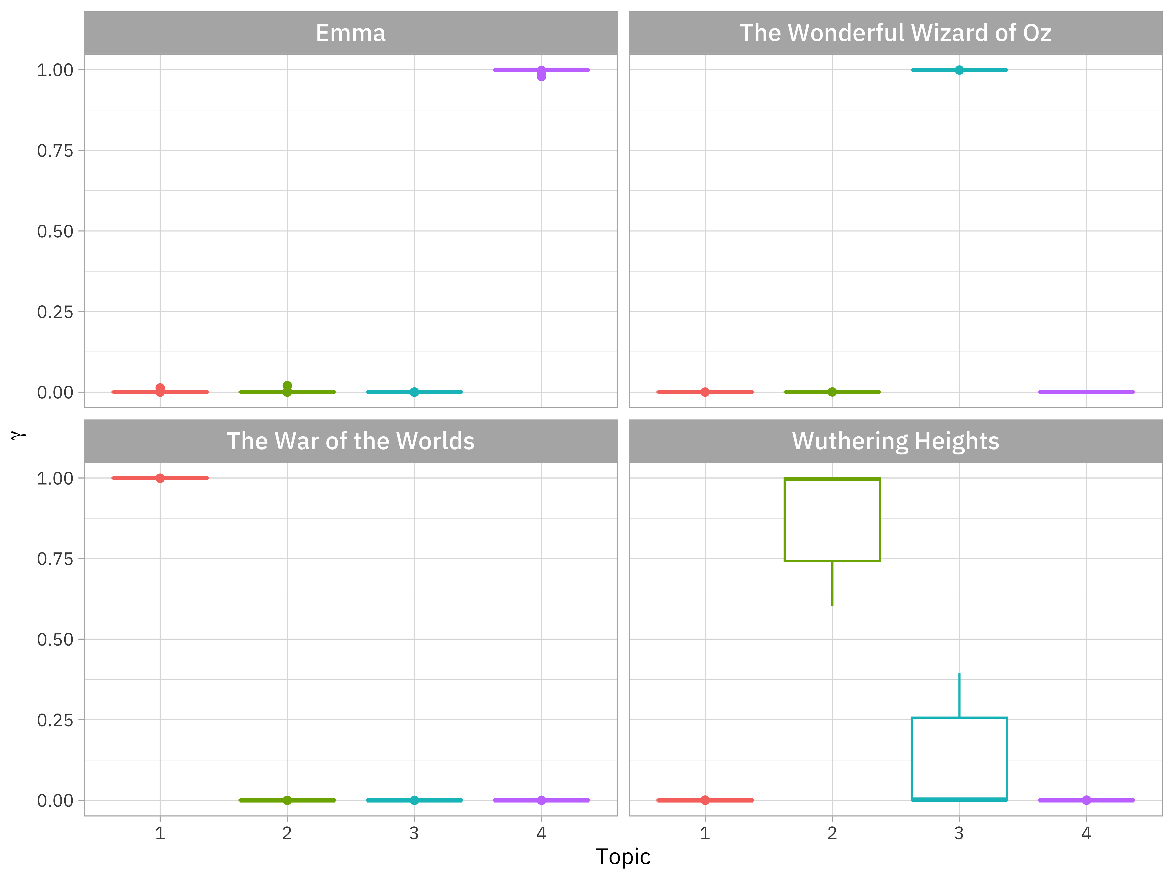
chapters_parsed |>

ggplot(aes(factor(topic), gamma)) +

facet_wrap(vars(title))

mutate(title = fct_reorder(title, gamma * topic)) |>

geom_boxplot() +
How are documents classified?

GOING FARTHER 🚀
Tidying model output
Which words in each document are assigned to which topics?
augment()- Add information to each observation in the original data
Using stm
- Document-level covariates
How do we choose \(K\)?😕
Use functions for
semanticCoherence(),checkResiduals(),exclusivity(), and more!Check out http://www.structuraltopicmodel.com/
Workflow for text mining/modeling
Thanks!

Slides created with Quarto