Text Mining

USING TIDY DATA PRINCIPLES

Julia Silge

Hello!

Let’s install some packages

install.packages(c("tidyverse", 
                   "tidytext",
                   "stopwords",
                   "gutenbergr"))

What do we mean by tidy text?

text <- c("Tell all the truth but tell it slant —",
          "Success in Circuit lies",
          "Too bright for our infirm Delight",
          "The Truth's superb surprise",
          "As Lightning to the Children eased",
          "With explanation kind",
          "The Truth must dazzle gradually",
          "Or every man be blind —")

text
#> [1] "Tell all the truth but tell it slant —"
#> [2] "Success in Circuit lies"               
#> [3] "Too bright for our infirm Delight"     
#> [4] "The Truth's superb surprise"           
#> [5] "As Lightning to the Children eased"    
#> [6] "With explanation kind"                 
#> [7] "The Truth must dazzle gradually"       
#> [8] "Or every man be blind —"

What do we mean by tidy text?

library(tidyverse)

text_df <- tibble(line = 1:8, text = text)

text_df
#> # A tibble: 8 × 2
#>    line text                                  
#>   <int> <chr>                                 
#> 1     1 Tell all the truth but tell it slant —
#> 2     2 Success in Circuit lies               
#> 3     3 Too bright for our infirm Delight     
#> 4     4 The Truth's superb surprise           
#> 5     5 As Lightning to the Children eased    
#> 6     6 With explanation kind                 
#> 7     7 The Truth must dazzle gradually       
#> 8     8 Or every man be blind —

What do we mean by tidy text?

library(tidytext)

text_df %>%
    unnest_tokens(word, text)
#> # A tibble: 41 × 2
#>     line word   
#>    <int> <chr>  
#>  1     1 tell   
#>  2     1 all    
#>  3     1 the    
#>  4     1 truth  
#>  5     1 but    
#>  6     1 tell   
#>  7     1 it     
#>  8     1 slant  
#>  9     2 success
#> 10     2 in     
#> # … with 31 more rows

Jane wants to know…

A tidy text dataset typically has

more
fewer

rows than the original, non-tidy text dataset.

Gathering more data

You can access the full text of many public domain works from Project Gutenberg using the gutenbergr package.

library(gutenbergr)

full_text <- gutenberg_download(1342, mirror = my_mirror)

What book do you want to analyze today? 📖🥳📖

Time to tidy your text!

tidy_book <- full_text %>%
    mutate(line = row_number()) %>%
    unnest_tokens(word, text)         

glimpse(tidy_book)
#> Rows: 127,996
#> Columns: 3
#> $ gutenberg_id <int> 1342, 1342, 1342, 1342, 1342, 1342, 1342, 1342, 1342, 134…
#> $ line         <int> 1, 3, 3, 4, 6, 6, 6, 6, 7, 9, 9, 12, 14, 14, 14, 14, 14, …
#> $ word         <chr> "illustration", "george", "allen", "publisher", "156", "c…

What are the most common words?

What do you predict will happen if we run the following code? 🤔

tidy_book %>%
    count(word, sort = TRUE)

What are the most common words?

What do you predict will happen if we run the following code? 🤔

tidy_book %>%
    count(word, sort = TRUE)
#> # A tibble: 7,118 × 2
#>    word      n
#>    <chr> <int>
#>  1 the    4656
#>  2 to     4323
#>  3 of     3838
#>  4 and    3763
#>  5 her    2260
#>  6 i      2095
#>  7 a      2036
#>  8 in     1991
#>  9 was    1871
#> 10 she    1732
#> # … with 7,108 more rows

Stop words

get_stopwords()
#> # A tibble: 175 × 2
#>    word      lexicon 
#>    <chr>     <chr>   
#>  1 i         snowball
#>  2 me        snowball
#>  3 my        snowball
#>  4 myself    snowball
#>  5 we        snowball
#>  6 our       snowball
#>  7 ours      snowball
#>  8 ourselves snowball
#>  9 you       snowball
#> 10 your      snowball
#> # … with 165 more rows

Stop words

get_stopwords(language = "es")
#> # A tibble: 308 × 2
#>    word  lexicon 
#>    <chr> <chr>   
#>  1 de    snowball
#>  2 la    snowball
#>  3 que   snowball
#>  4 el    snowball
#>  5 en    snowball
#>  6 y     snowball
#>  7 a     snowball
#>  8 los   snowball
#>  9 del   snowball
#> 10 se    snowball
#> # … with 298 more rows

Stop words

get_stopwords(language = "fr")
#> # A tibble: 164 × 2
#>    word  lexicon 
#>    <chr> <chr>   
#>  1 au    snowball
#>  2 aux   snowball
#>  3 avec  snowball
#>  4 ce    snowball
#>  5 ces   snowball
#>  6 dans  snowball
#>  7 de    snowball
#>  8 des   snowball
#>  9 du    snowball
#> 10 elle  snowball
#> # … with 154 more rows

Stop words

get_stopwords(source = "smart")
#> # A tibble: 571 × 2
#>    word        lexicon
#>    <chr>       <chr>  
#>  1 a           smart  
#>  2 a's         smart  
#>  3 able        smart  
#>  4 about       smart  
#>  5 above       smart  
#>  6 according   smart  
#>  7 accordingly smart  
#>  8 across      smart  
#>  9 actually    smart  
#> 10 after       smart  
#> # … with 561 more rows

What are the most common words?

U N S C R A M B L E

anti_join(get_stopwords(source = “smart”)) %>%

tidy_book %>%

count(word, sort = TRUE) %>%

geom_col() +

slice_max(n, n = 20) %>%

ggplot(aes(n, fct_reorder(word, n))) +

What are the most common words?

tidy_book %>%
    anti_join(get_stopwords(source = "smart")) %>%
    count(word, sort = TRUE) %>%
    slice_max(n, n = 20) %>%
    ggplot(aes(n, fct_reorder(word, n))) +  
    geom_col()

SENTIMENT ANALYSIS
😄😢😠

Sentiment lexicons

get_sentiments("afinn")
#> # A tibble: 2,477 × 2
#>    word       value
#>    <chr>      <dbl>
#>  1 abandon       -2
#>  2 abandoned     -2
#>  3 abandons      -2
#>  4 abducted      -2
#>  5 abduction     -2
#>  6 abductions    -2
#>  7 abhor         -3
#>  8 abhorred      -3
#>  9 abhorrent     -3
#> 10 abhors        -3
#> # … with 2,467 more rows

Sentiment lexicons

get_sentiments("bing")
#> # A tibble: 6,786 × 2
#>    word        sentiment
#>    <chr>       <chr>    
#>  1 2-faces     negative 
#>  2 abnormal    negative 
#>  3 abolish     negative 
#>  4 abominable  negative 
#>  5 abominably  negative 
#>  6 abominate   negative 
#>  7 abomination negative 
#>  8 abort       negative 
#>  9 aborted     negative 
#> 10 aborts      negative 
#> # … with 6,776 more rows

Sentiment lexicons

get_sentiments("nrc")
#> # A tibble: 13,872 × 2
#>    word        sentiment
#>    <chr>       <chr>    
#>  1 abacus      trust    
#>  2 abandon     fear     
#>  3 abandon     negative 
#>  4 abandon     sadness  
#>  5 abandoned   anger    
#>  6 abandoned   fear     
#>  7 abandoned   negative 
#>  8 abandoned   sadness  
#>  9 abandonment anger    
#> 10 abandonment fear     
#> # … with 13,862 more rows

Sentiment lexicons

get_sentiments("loughran")
#> # A tibble: 4,150 × 2
#>    word         sentiment
#>    <chr>        <chr>    
#>  1 abandon      negative 
#>  2 abandoned    negative 
#>  3 abandoning   negative 
#>  4 abandonment  negative 
#>  5 abandonments negative 
#>  6 abandons     negative 
#>  7 abdicated    negative 
#>  8 abdicates    negative 
#>  9 abdicating   negative 
#> 10 abdication   negative 
#> # … with 4,140 more rows

Implementing sentiment analysis

tidy_book %>%
    inner_join(get_sentiments("bing")) %>% 
    count(sentiment, sort = TRUE)
#> # A tibble: 2 × 2
#>   sentiment     n
#>   <chr>     <int>
#> 1 positive   5306
#> 2 negative   3864

Jane wants to know…

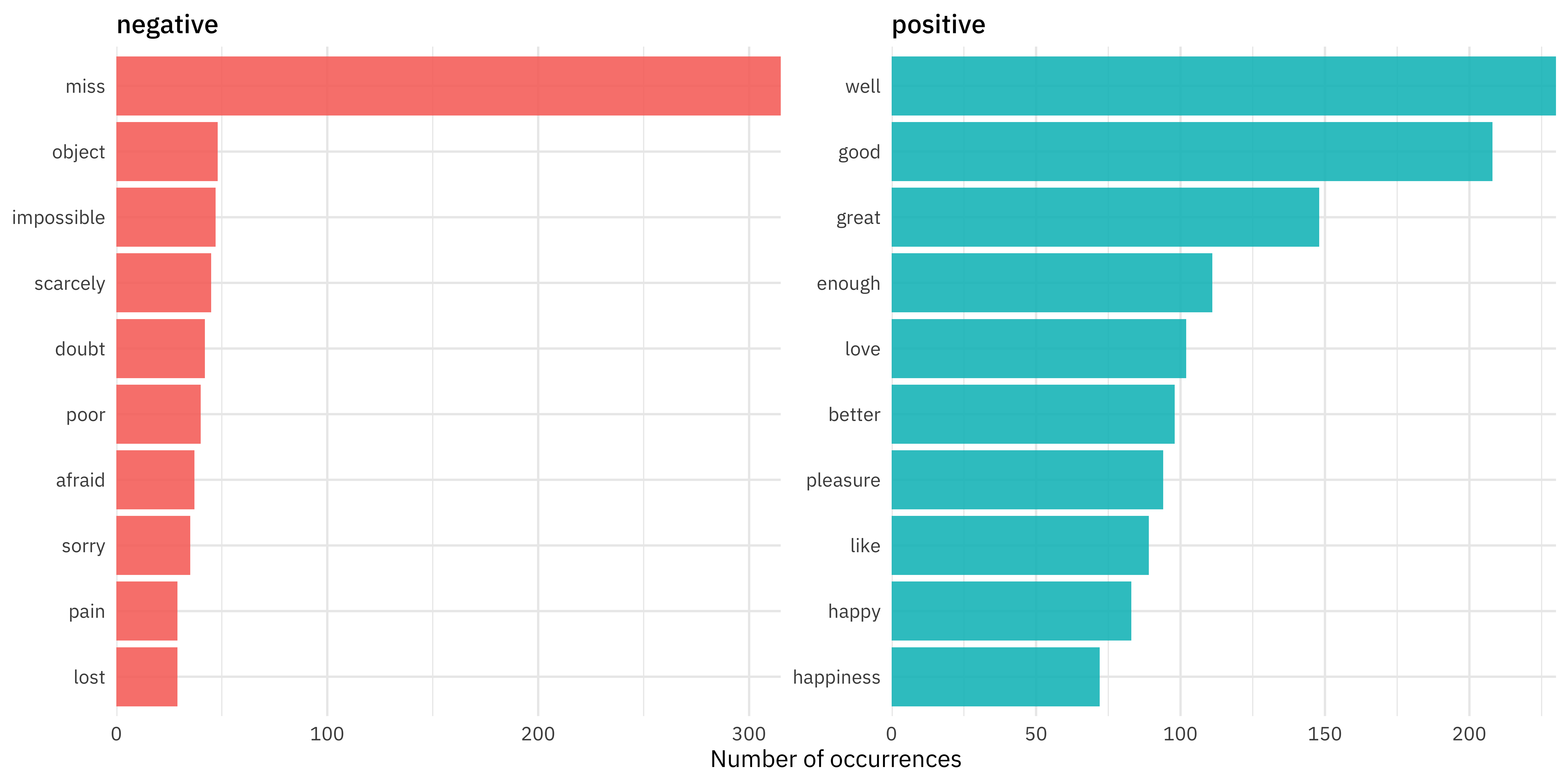
What kind of join is appropriate for sentiment analysis?

anti_join()
full_join()
outer_join()
inner_join()

Implementing sentiment analysis

What do you predict will happen if we run the following code? 🤔

tidy_book %>%
    inner_join(get_sentiments("bing")) %>%            
    count(sentiment, word, sort = TRUE)

Implementing sentiment analysis

What do you predict will happen if we run the following code? 🤔

tidy_book %>%
    inner_join(get_sentiments("bing")) %>%            
    count(sentiment, word, sort = TRUE)   
#> # A tibble: 1,503 × 3
#>    sentiment word         n
#>    <chr>     <chr>    <int>
#>  1 negative  miss       315
#>  2 positive  well       230
#>  3 positive  good       208
#>  4 positive  great      148
#>  5 positive  enough     111
#>  6 positive  love       102
#>  7 positive  better      98
#>  8 positive  pleasure    94
#>  9 positive  like        89
#> 10 positive  happy       83
#> # … with 1,493 more rows

Implementing sentiment analysis

tidy_book %>%
    inner_join(get_sentiments("bing")) %>%
    count(sentiment, word, sort = TRUE) %>%
    group_by(sentiment) %>%
    slice_max(n, n = 10) %>%
    ungroup() %>%
    ggplot(aes(n, fct_reorder(word, n), fill = sentiment)) +
    geom_col() +
    facet_wrap(vars(sentiment), scales = "free")

Thanks!

@juliasilge

youtube.com/juliasilge

juliasilge.com

tidytextmining.com

Text Mining

Hello!

Let’s install some packages

What do we mean by tidy text?

What do we mean by tidy text?

What do we mean by tidy text?

Jane wants to know…

Gathering more data

Time to tidy your text!

What are the most common words?

What are the most common words?

Stop words

Stop words

Stop words

Stop words

Stop words

What are the most common words?

What are the most common words?

SENTIMENT ANALYSIS 😄😢😠

Sentiment lexicons

Sentiment lexicons

Sentiment lexicons

Sentiment lexicons

Implementing sentiment analysis

Jane wants to know…

Implementing sentiment analysis

Implementing sentiment analysis

Implementing sentiment analysis

Thanks!

SENTIMENT ANALYSIS
😄😢😠