Text Mining
USING TIDY DATA PRINCIPLES
Hello!
Let’s install some packages
WHAT IS A DOCUMENT ABOUT? 🤔
What is a document about?
- Term frequency
- Inverse document frequency
\[idf(\text{term}) = \ln{\left(\frac{n_{\text{documents}}}{n_{\text{documents containing term}}}\right)}\]
tf-idf is about comparing documents within a collection.
Understanding tf-idf
Make a collection (corpus) for yourself! 💅
Understanding tf-idf
Make a collection (corpus) for yourself! 💅
full_collection
#> # A tibble: 59,360 × 3
#>    gutenberg_id text             title
#>           <int> <chr>            <chr>
#>  1          141 "MANSFIELD PARK" Mansfield Park
#>  2          141 ""               Mansfield Park
#>  3          141 "(1814)"         Mansfield Park
#>  4          141 ""               Mansfield Park
#>  5          141 "By Jane Austen" Mansfield Park
#>  6          141 ""               Mansfield Park
#>  7          141 ""               Mansfield Park
#>  8          141 "Contents"       Mansfield Park
#>  9          141 ""               Mansfield Park
#> 10          141 "   CHAPTER I"   Mansfield Park
#> # … with 59,350 more rows
Counting word frequencies
What do the columns of book_words tell us?
Calculating tf-idf
Calculating tf-idf
book_tf_idf
#> # A tibble: 29,055 × 6
#>    title               word      n     tf   idf tf_idf
#>    <chr>               <chr> <int>  <dbl> <dbl>  <dbl>
#>  1 Mansfield Park      the    6207 0.0387     0      0
#>  2 Mansfield Park      to     5473 0.0341     0      0
#>  3 Mansfield Park      and    5437 0.0339     0      0
#>  4 Emma                to     5238 0.0325     0      0
#>  5 Emma                the    5201 0.0323     0      0
#>  6 Emma                and    4896 0.0304     0      0
#>  7 Mansfield Park      of     4777 0.0298     0      0
#>  8 Pride and Prejudice the    4656 0.0364     0      0
#>  9 Pride and Prejudice to     4323 0.0338     0      0
#> 10 Emma                of     4291 0.0266     0      0
#> # … with 29,045 more rows
That’s… super exciting???
Calculating tf-idf
What do you predict will happen if we run the following code? 🤔
Calculating tf-idf
What do you predict will happen if we run the following code? 🤔
book_tf_idf %>%
    arrange(-tf_idf)
#> # A tibble: 29,055 × 6
#> title word n tf idf tf_idf
#> <chr> <chr> <int> <dbl> <dbl> <dbl>
#> 1 Sense and Sensibility elinor 622 0.00518 1.39 0.00718
#> 2 Sense and Sensibility marianne 492 0.00410 1.39 0.00568
#> 3 Pride and Prejudice darcy 383 0.00299 1.39 0.00415
#> 4 Emma emma 786 0.00488 0.693 0.00338
#> 5 Pride and Prejudice bennet 309 0.00241 1.39 0.00335
#> 6 Emma weston 388 0.00241 1.39 0.00334
#> 7 Pride and Prejudice elizabeth 605 0.00473 0.693 0.00328
#> 8 Emma knightley 356 0.00221 1.39 0.00306
#> 9 Pride and Prejudice bingley 262 0.00205 1.39 0.00284
#> 10 Emma elton 319 0.00198 1.39 0.00274
#> # … with 29,045 more rowsCalculating tf-idf
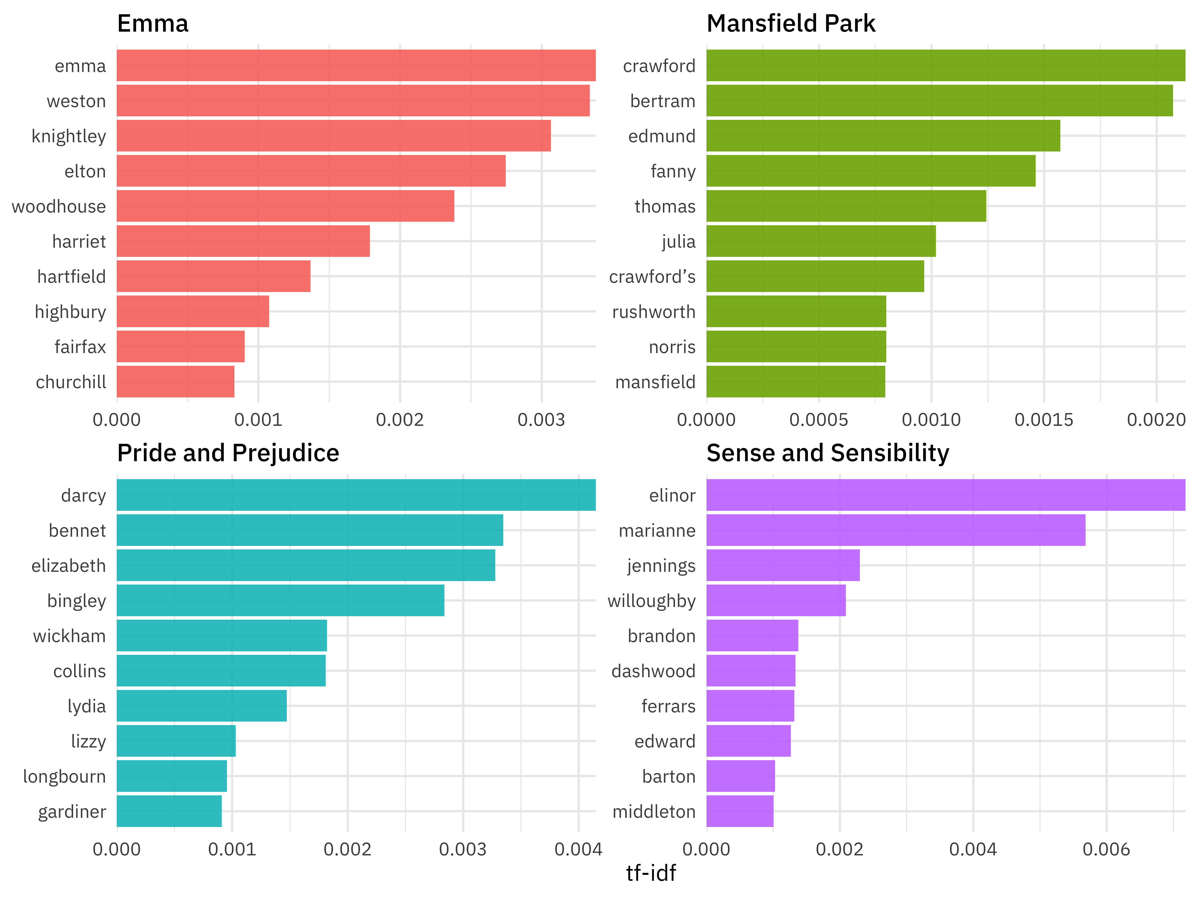
U N S C R A M B L E
group_by(title) %>%
book_tf_idf %>%
slice_max(tf_idf, n = 10) %>%
ggplot(aes(tf_idf, fct_reorder(word, tf_idf), fill = title)) +
facet_wrap(vars(title), scales = “free”)
geom_col(show.legend = FALSE) +
Calculating tf-idf
WHAT IS A DOCUMENT ABOUT? 🤔
What is a document about?
- Term frequency
- Inverse document frequency
Weighted log odds ⚖️
- Log odds ratio expresses probabilities
- Weighting helps deal with power law distribution
Weighted log odds ⚖️
library(tidylo)
book_words %>%
    bind_log_odds(title, word, n) %>%
    arrange(-log_odds_weighted)
#> # A tibble: 29,055 × 4
#>    title                 word          n log_odds_weighted
#>    <chr>                 <chr>     <int>             <dbl>
#>  1 Sense and Sensibility elinor      622              35.6
#>  2 Sense and Sensibility marianne    492              31.6
#>  3 Emma                  emma        786              29.3
#>  4 Pride and Prejudice   darcy       383              27.5
#>  5 Pride and Prejudice   elizabeth   605              26.9
#>  6 Emma                  weston      388              26.8
#>  7 Emma                  knightley   356              25.7
#>  8 Pride and Prejudice   bennet      309              24.7
#>  9 Emma                  elton       319              24.3
#> 10 Mansfield Park        crawford    493              23.2
#> # … with 29,045 more rows
Weighted log odds can distinguish between words that are used in all texts.
N-GRAMS… AND BEYOND! 🚀
N-grams… and beyond! 🚀
N-grams… and beyond! 🚀
tidy_ngram
#> # A tibble: 147,256 × 2
#>    gutenberg_id bigram
#>           <int> <chr>
#>  1          158 by jane
#>  2          158 jane austen
#>  3          158 volume i
#>  4          158 chapter i
#>  5          158 chapter ii
#>  6          158 chapter iii
#>  7          158 chapter iv
#>  8          158 chapter v
#>  9          158 chapter vi
#> 10          158 chapter vii
#> # … with 147,246 more rows
N-grams… and beyond! 🚀
Jane wants to know…
Can we use an anti_join() now to remove stop words?
- Yes! ✅
- No ☹️
N-grams… and beyond! 🚀
N-grams… and beyond! 🚀
bigram_counts
#> # A tibble: 6,526 × 3
#>    word1 word2         n
#>    <chr> <chr>     <int>
#>  1 miss  woodhouse   136
#>  2 frank churchill   110
#>  3 miss  fairfax     101
#>  4 miss  bates        95
#>  5 jane  fairfax      90
#>  6 john  knightley    47
#>  7 miss  smith        45
#>  8 miss  taylor       39
#>  9 dear  emma         30
#> 10 maple grove        28
#> # … with 6,516 more rows
What can you do with n-grams?
- tf-idf of n-grams
- weighted log odds of n-grams
- network analysis
- negation
https://pudding.cool/2017/08/screen-direction/
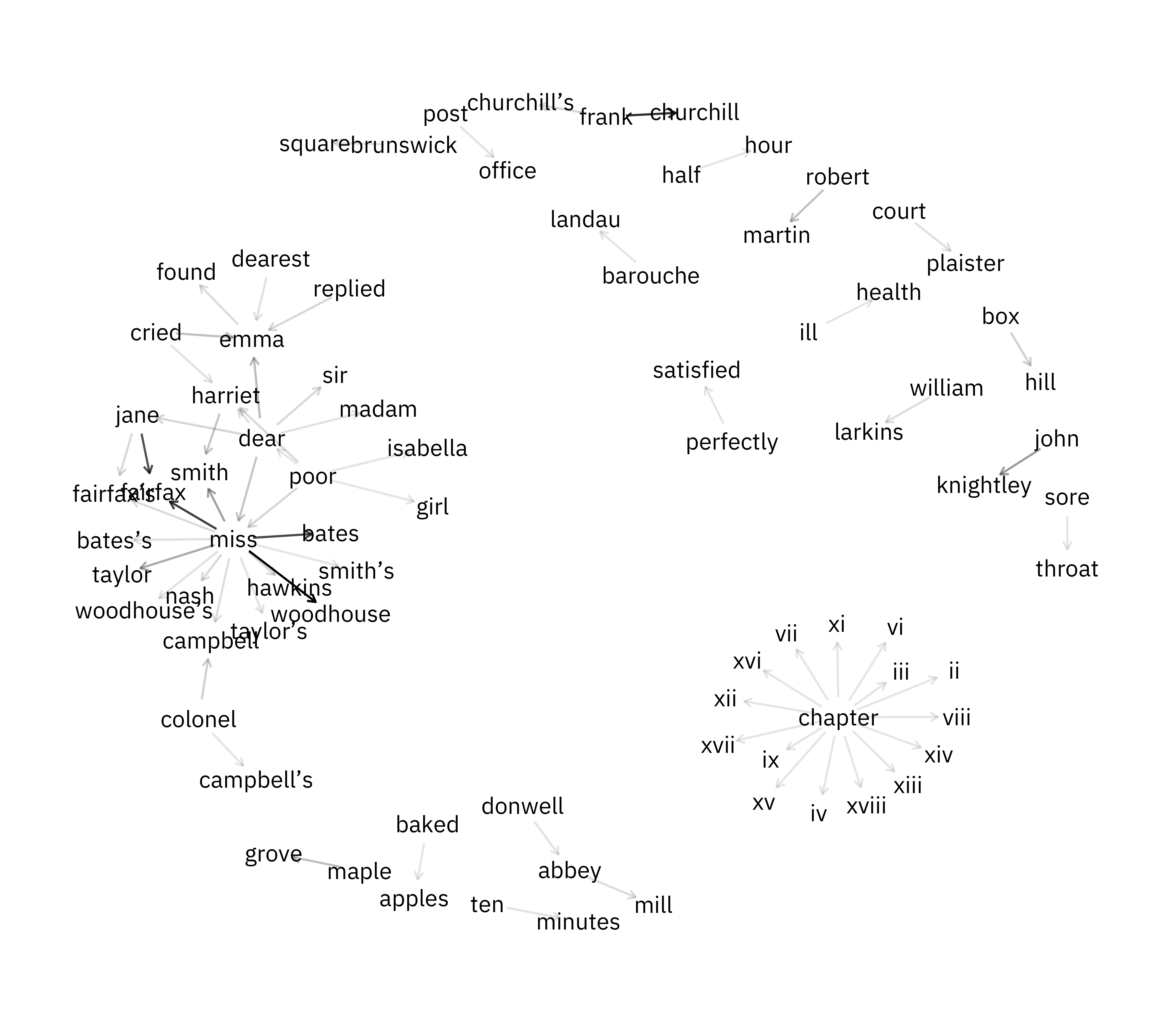
Network analysis
Network analysis
bigram_graph
#> # A tbl_graph: 81 nodes and 68 edges
#> #
#> # A directed acyclic simple graph with 19 components
#> #
#> # Node Data: 81 × 1 (active)
#>   name
#>   <chr>
#> 1 miss
#> 2 frank
#> 3 jane
#> 4 john
#> 5 dear
#> 6 maple
#> # … with 75 more rows
#> #
#> # Edge Data: 68 × 3
#>    from    to     n
#>   <int> <int> <int>
#> 1     1    30   136
#> 2     2    31   110
#> 3     1    32   101
#> # … with 65 more rows
Jane wants to know…
Is bigram_graph a tidy dataset?
- Yes ☑️
- No 🚫
Network analysis
Network analysis
Thanks!
Slides created with Quarto