Text Mining
USING TIDY DATA PRINCIPLES
Hello!

Let’s install some packages
Workflow for text mining/modeling
Topic modeling
📖 Each DOCUMENT = mixture of topics
📑 Each TOPIC = mixture of tokens
GREAT LIBRARY HEIST 🕵
Download your text data
library(tidyverse)
library(gutenbergr)

books <- gutenberg_download(c(36, 158, 164, 345),
                            meta_fields = "title",
                            mirror = my_mirror)
books %>%
    count(title)
#> # A tibble: 4 × 2
#>   title                                     n
#>   <chr>                                 <int>
#> 1 Dracula                               15480
#> 2 Emma                                  16488
#> 3 The War of the Worlds                  6372
#> 4 Twenty Thousand Leagues under the Sea 12426
Someone has torn up your books! 😭
What do you predict will happen if we run the following code? 🤔
Someone has torn up your books! 😭
What do you predict will happen if we run the following code? 🤔
books_by_document <- books %>%
    group_by(title) %>%
    mutate(document = row_number() %/% 500) %>%
    ungroup() %>%
    unite(document, title, document)

glimpse(books_by_document)
#> Rows: 50,766
#> Columns: 3
#> $ gutenberg_id <int> 36, 36, 36, 36, 36, 36, 36, 36, 36, 36, 36, 36, 36, 36, 3…
#> $ text <chr> "cover ", "", "", "", "", "The War of the Worlds", "", "b…
#> $ document <chr> "The War of the Worlds_0", "The War of the Worlds_0", "Th…Can we put them back together?
library(tidytext)
word_counts <- books_by_document %>%
    unnest_tokens(word, text) %>%
    anti_join(get_stopwords(source = "smart")) %>%
    count(document, word, sort = TRUE)

glimpse(word_counts)
#> Rows: 100,572
#> Columns: 3
#> $ document <chr> "Emma_0", "Emma_7", "Emma_2", "Emma_8", "Emma_11", "Emma_6", …
#> $ word     <chr> "chapter", "mr", "mr", "mr", "mr", "mr", "mr", "chapter", "mr…
#> $ n        <int> 57, 56, 54, 52, 51, 50, 49, 49, 48, 44, 44, 43, 43, 42, 42, 4…
Jane wants to know…

The dataset word_counts contains
- the counts of words per book
- the counts of words per “chunk” (500 lines)
- the counts of words per line
Can we put them back together?
Jane wants to know…

Is words_sparse a tidy dataset?
- Yes ✔️
- No 🚫
Train a topic model
Use a sparse matrix or a quanteda::dfm object as input
Train a topic model
Use a sparse matrix or a quanteda::dfm object as input
summary(topic_model)
#> A topic model with 4 topics, 102 documents and a 18370 word dictionary.
#> Topic 1 Top Words:
#>       Highest Prob: mr, emma, harriet, good, miss, thing, man
#>       FREX: charade, taylor, papa, isabella, martin, children, marry
#>       Lift: charade, monarch, hannah, hating, humours, militia, widower
#>       Score: emma, harriet, knightley, elton, weston, hartfield, martin
#> Topic 2 Top Words:
#>       Highest Prob: captain, _nautilus_, sea, nemo, ned, conseil, land
#>       FREX: _nautilus_, nemo, ned, conseil, ocean, canadian, submarine
#>       Lift: natives, astrolabe, canoes, galleons, gallons, morses, dillon
#>       Score: _nautilus_, nemo, ned, conseil, captain, canadian, ocean
#> Topic 3 Top Words:
#>       Highest Prob: mr, mrs, emma, miss, weston, thing, jane
#>       FREX: campbell, dixon, grove, maple, fairfax’s, engagement, jane
#>       Lift: ford, larkins, patty, ford’s, sucklings, coxes, hodges
#>       Score: emma, weston, jane, knightley, harriet, elton, mrs
#> Topic 4 Top Words:
#>       Highest Prob: time, night, man, back, van, helsing, day
#>       FREX: helsing, lucy, mina, jonathan, martians, harker, diary
#>       Lift: scullery, boxes, skinsky, wolves, ogilvy, renfield, galatz
#>       Score: helsing, martians, lucy, mina, van, jonathan, diary
Explore the topic model output
chapter_topics <- tidy(topic_model, matrix = "beta")
chapter_topics
#> # A tibble: 73,480 × 3
#>    topic term        beta
#>    <int> <chr>      <dbl>
#>  1     1 chapter 5.88e- 3
#>  2     2 chapter 2.11e- 3
#>  3     3 chapter 8.87e- 4
#>  4     4 chapter 6.80e- 4
#>  5     1 mr      2.82e- 2
#>  6     2 mr      2.23e- 4
#>  7     3 mr      1.96e- 2
#>  8     4 mr      9.58e- 4
#>  9     1 mrs     5.17e- 3
#> 10     2 mrs     3.90e-42
#> # … with 73,470 more rows
Explore the topic model output
U N S C R A M B L E
top_terms <- chapter_topics %>%
ungroup() %>%
group_by(topic) %>%
arrange(topic, -beta)
slice_max(beta, n = 10) %>%
Explore the topic model output
Explore the topic model output
top_terms
#> # A tibble: 40 × 3
#>    topic term         beta
#>    <int> <chr>       <dbl>
#>  1     1 mr        0.0282
#>  2     1 emma      0.0125
#>  3     1 harriet   0.0115
#>  4     1 good      0.0105
#>  5     1 miss      0.00914
#>  6     1 thing     0.00787
#>  7     1 man       0.00764
#>  8     1 knightley 0.00696
#>  9     1 elton     0.00680
#> 10     1 dear      0.00633
#> # … with 30 more rows
Explore the topic model output

Identify important words
⭐ FREX
⬆️ LIFT
High FREX words
High frequency and high exclusivity
High lift words
Topic-word distribution divided by word count distribution
How are documents classified?
chapters_gamma <- tidy(topic_model, matrix = "gamma",
                       document_names = rownames(words_sparse))
chapters_gamma
#> # A tibble: 408 × 3
#>    document                                topic    gamma
#>    <chr>                                   <int>    <dbl>
#>  1 Emma_0                                      1 0.999
#>  2 Emma_7                                      1 0.239
#>  3 Emma_2                                      1 0.999
#>  4 Emma_8                                      1 0.233
#>  5 Emma_11                                     1 0.00103
#>  6 Emma_6                                      1 0.999
#>  7 Emma_21                                     1 0.000715
#>  8 Twenty Thousand Leagues under the Sea_0     1 0.000146
#>  9 Emma_20                                     1 0.000937
#> 10 Emma_19                                     1 0.000977
#> # … with 398 more rows
How are documents classified?
What do you predict will happen if we run the following code? 🤔
How are documents classified?
What do you predict will happen if we run the following code? 🤔
chapters_parsed <- chapters_gamma %>%
    separate(document, c("title", "chapter"),
             sep = "_", convert = TRUE)

glimpse(chapters_parsed)
#> Rows: 408
#> Columns: 4
#> $ title <chr> "Emma", "Emma", "Emma", "Emma", "Emma", "Emma", "Emma", "Twent…
#> $ chapter <int> 0, 7, 2, 8, 11, 6, 21, 0, 20, 19, 4, 9, 15, 21, 23, 27, 19, 14…
#> $ topic <int> 1, 1, 1, 1, 1, 1, 1, 1, 1, 1, 1, 1, 1, 1, 1, 1, 1, 1, 1, 1, 1,…
#> $ gamma <dbl> 9.986350e-01, 2.387502e-01, 9.988524e-01, 2.325374e-01, 1.0326…How are documents classified?
U N S C R A M B L E
chapters_parsed %>%
ggplot(aes(factor(topic), gamma)) +
facet_wrap(vars(title))
mutate(title = fct_reorder(title, gamma * topic)) %>%
geom_boxplot() +
How are documents classified?

GOING FARTHER 🚀
Tidying model output
Which words in each document are assigned to which topics?
augment()- Add information to each observation in the original data
Using stm
- Document-level covariates
Use functions for
semanticCoherence(),checkResiduals(),exclusivity(), and more!Check out http://www.structuraltopicmodel.com/
Stemming?
“Comparing Apples to Apple: The Effects of Stemmers on Topic Models”:
Despite their frequent use in topic modeling, we find that stemmers produce no meaningful improvement in likelihood and coherence and in fact can degrade topic stability.
HOW DO WE CHOOSE \(K\)? 😕
Train many topic models
Train many topic models
heldout <- make.heldout(words_sparse)

k_result <- many_models %>%
    mutate(exclusivity        = map(topic_model, exclusivity),
           semantic_coherence = map(topic_model, semanticCoherence, words_sparse),
           eval_heldout       = map(topic_model, eval.heldout, heldout$missing),
           residual           = map(topic_model, checkResiduals, words_sparse),
           bound              = map_dbl(topic_model, function(x) max(x$convergence$bound)),
           lfact              = map_dbl(topic_model, function(x) lfactorial(x$settings$dim$K)),
           lbound             = bound + lfact,
           iterations         = map_dbl(topic_model, function(x) length(x$convergence$bound)))
Train many topic models
k_result
#> # A tibble: 5 × 10
#> K topic_…¹ exclu…² seman…³ eval_heldout residual bound lfact lbound
#> <dbl> <list> <list> <list> <list> <list> <dbl> <dbl> <dbl>
#> 1 3 <STM> <dbl> <dbl> <named list> <named list> -1.40e6 1.79 -1.40e6
#> 2 4 <STM> <dbl> <dbl> <named list> <named list> -1.39e6 3.18 -1.39e6
#> 3 6 <STM> <dbl> <dbl> <named list> <named list> -1.37e6 6.58 -1.37e6
#> 4 8 <STM> <dbl> <dbl> <named list> <named list> -1.35e6 10.6 -1.35e6
#> 5 10 <STM> <dbl> <dbl> <named list> <named list> -1.34e6 15.1 -1.34e6
#> # … with 1 more variable: iterations <dbl>, and abbreviated variable names
#> # ¹topic_model, ²exclusivity, ³semantic_coherenceTrain many topic models
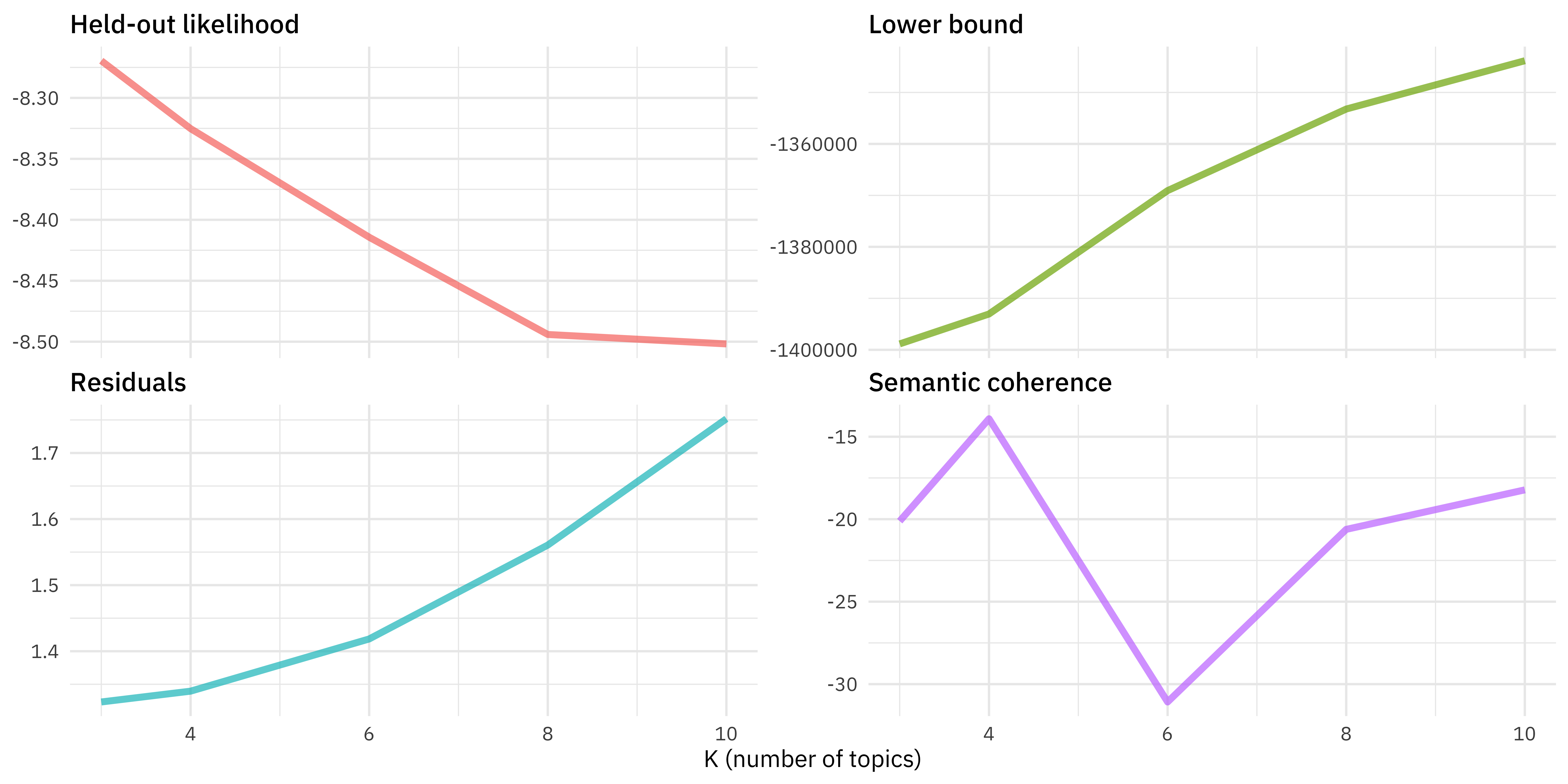
k_result %>%
    transmute(K,
              `Lower bound`         = lbound,
              Residuals             = map_dbl(residual, "dispersion"),
              `Semantic coherence`  = map_dbl(semantic_coherence, mean),
              `Held-out likelihood` = map_dbl(eval_heldout, "expected.heldout")) %>%
    gather(Metric, Value, -K) %>%
    ggplot(aes(K, Value, color = Metric)) +
    geom_line() +
    facet_wrap(~Metric, scales = "free_y")
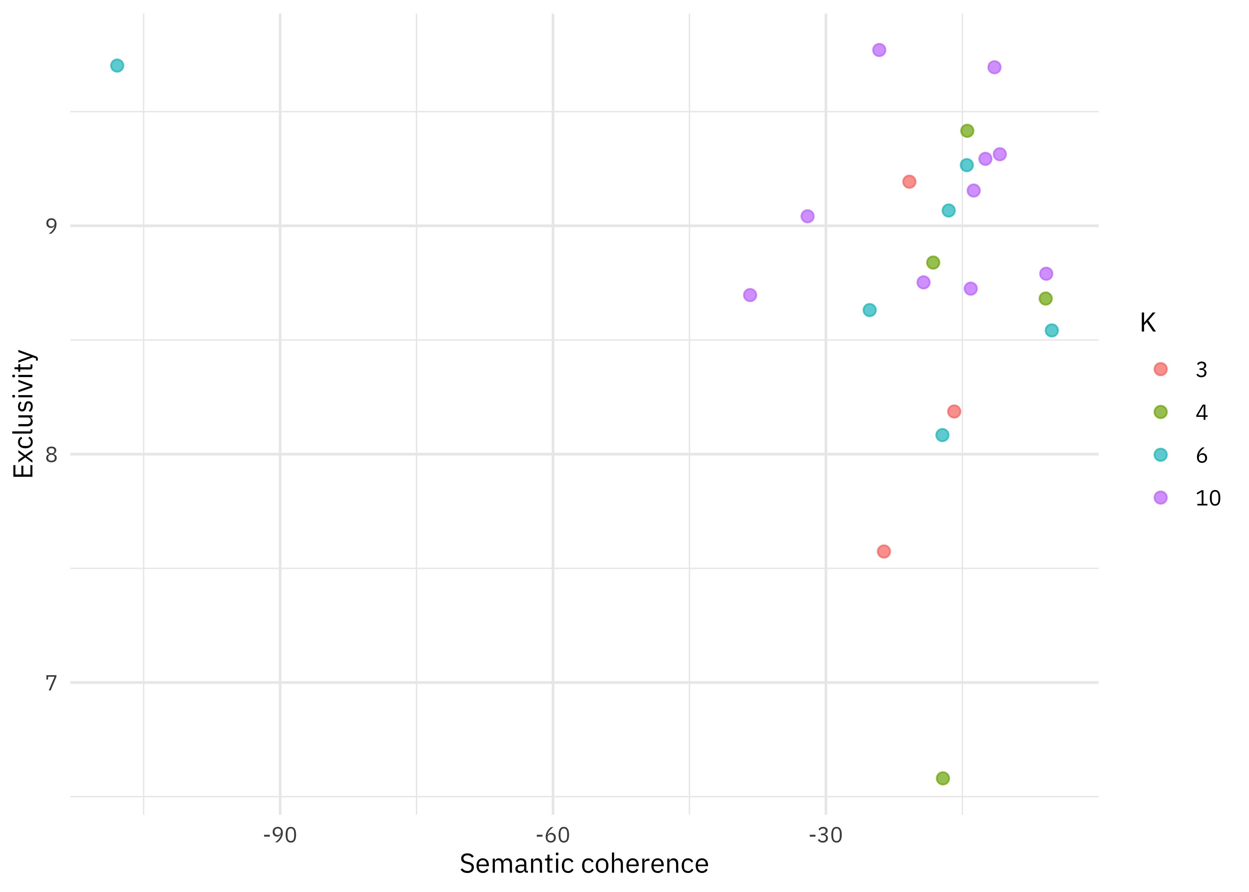
What is semantic coherence?
Semantic coherence is maximized when the most probable words in a given topic frequently co-occur together
Correlates well with human judgment of topic quality 😃
Having high semantic coherence is relatively easy, though, if you only have a few topics dominated by very common words 😩
Measure semantic coherence and exclusivity
Train many topic models

Jane wants to know…

Topic modeling is an example of…
- supervised machine learning
- unsupervised machine learning
Workflow for text mining/modeling
Go explore real-world text!
Thanks!

Slides created with Quarto