Tidiers for Structural Topic Models from the stm package

Tidy topic models fit by the stm package. The arguments and return values are similar to lda_tidiers().

# S3 method for STM
tidy(
  x,
  matrix = c("beta", "gamma", "theta", "frex", "lift"),
  log = FALSE,
  document_names = NULL,
  ...
)

# S3 method for estimateEffect
tidy(x, ...)

# S3 method for estimateEffect
glance(x, ...)

# S3 method for STM
augment(x, data, ...)

# S3 method for STM
glance(x, ...)

Arguments

x

An STM fitted model object from either stm::stm() or stm::estimateEffect()

matrix

Which matrix to tidy:

the beta matrix (per-term-per-topic, default)
the gamma/theta matrix (per-document-per-topic); the stm package calls this the theta matrix, but other topic modeling packages call this gamma
the FREX matrix, for words with high frequency and exclusivity
the lift matrix, for words with high lift

log

Whether beta/gamma/theta should be on a log scale, default FALSE

document_names

Optional vector of document names for use with per-document-per-topic tidying

...

Extra arguments for tidying, such as w as used in stm::calcfrex()

data

For augment, the data given to the stm function, either as a dfm from quanteda or as a tidied table with "document" and "term" columns

Value

tidy returns a tidied version of either the beta, gamma, FREX, or lift matrix if called on an object from stm::stm(), or a tidied version of the estimated regressions if called on an object from stm::estimateEffect().

glance returns a tibble with exactly one row of model summaries.

augment must be provided a data argument, either a dfm from quanteda or a table containing one row per original document-term pair, such as is returned by tdm_tidiers, containing columns document and term. It returns that same data with an additional column .topic with the topic assignment for that document-term combination.

Examples

library(dplyr)
library(ggplot2)
library(stm)
#> stm v1.3.7 successfully loaded. See ?stm for help. 
#>  Papers, resources, and other materials at structuraltopicmodel.com
library(janeaustenr)

austen_sparse <- austen_books() %>%
    unnest_tokens(word, text) %>%
    anti_join(stop_words) %>%
    count(book, word) %>%
    cast_sparse(book, word, n)
#> Joining with `by = join_by(word)`
topic_model <- stm(austen_sparse, K = 12, verbose = FALSE)

# tidy the word-topic combinations
td_beta <- tidy(topic_model)
td_beta
#> # A tibble: 166,968 × 3
#>    topic term      beta
#>    <int> <chr>    <dbl>
#>  1     1 1     1.18e- 4
#>  2     2 1     1.15e-19
#>  3     3 1     5.51e- 5
#>  4     4 1     1.33e-19
#>  5     5 1     4.20e- 5
#>  6     6 1     2.68e- 5
#>  7     7 1     4.20e- 5
#>  8     8 1     1.18e- 4
#>  9     9 1     4.20e- 5
#> 10    10 1     4.20e- 5
#> # ℹ 166,958 more rows

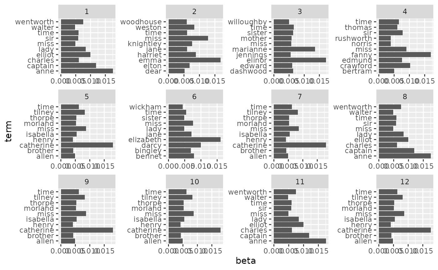
# Examine the topics
td_beta %>%
    group_by(topic) %>%
    slice_max(beta, n = 10) %>%
    ungroup() %>%
    ggplot(aes(beta, term)) +
    geom_col() +
    facet_wrap(~ topic, scales = "free")


# high FREX words per topic
tidy(topic_model, matrix = "frex")
#> # A tibble: 166,968 × 2
#>    topic term      
#>    <int> <chr>     
#>  1     1 elliot    
#>  2     1 wentworth 
#>  3     1 walter    
#>  4     1 anne      
#>  5     1 russell   
#>  6     1 musgrove  
#>  7     1 louisa    
#>  8     1 charles   
#>  9     1 uppercross
#> 10     1 kellynch  
#> # ℹ 166,958 more rows

# high lift words per topic
tidy(topic_model, matrix = "lift")
#> # A tibble: 166,968 × 2
#>    topic term           
#>    <int> <chr>          
#>  1     1 acknowledgement
#>  2     1 lyme           
#>  3     1 musgrove       
#>  4     1 walter         
#>  5     1 benwick        
#>  6     1 henrietta      
#>  7     1 kellynch       
#>  8     1 russell        
#>  9     1 uppercross     
#> 10     1 harville       
#> # ℹ 166,958 more rows

# tidy the document-topic combinations, with optional document names
td_gamma <- tidy(topic_model, matrix = "gamma",
                 document_names = rownames(austen_sparse))
td_gamma
#> # A tibble: 72 × 3
#>    document            topic      gamma
#>    <chr>               <int>      <dbl>
#>  1 Sense & Sensibility     1 0.00000260
#>  2 Pride & Prejudice       1 0.00000279
#>  3 Mansfield Park          1 0.00000268
#>  4 Emma                    1 0.00000230
#>  5 Northanger Abbey        1 0.00000761
#>  6 Persuasion              1 0.333     
#>  7 Sense & Sensibility     2 0.00000472
#>  8 Pride & Prejudice       2 0.00000483
#>  9 Mansfield Park          2 0.00000393
#> 10 Emma                    2 1.00      
#> # ℹ 62 more rows

# using stm's gardarianFit, we can tidy the result of a model
# estimated with covariates
effects <- estimateEffect(1:3 ~ treatment, gadarianFit, gadarian)
glance(effects)
#> # A tibble: 1 × 3
#>       k  docs uncertainty
#>   <int> <int> <chr>      
#> 1     3   341 Global     
td_estimate <- tidy(effects)
td_estimate
#> # A tibble: 6 × 6
#>   topic term        estimate std.error statistic  p.value
#>   <int> <chr>          <dbl>     <dbl>     <dbl>    <dbl>
#> 1     1 (Intercept)   0.437     0.0241     18.1  1.13e-51
#> 2     1 treatment    -0.153     0.0322     -4.75 3.00e- 6
#> 3     2 (Intercept)   0.212     0.0224      9.44 6.18e-19
#> 4     2 treatment     0.242     0.0331      7.31 1.93e-12
#> 5     3 (Intercept)   0.351     0.0231     15.2  2.57e-40
#> 6     3 treatment    -0.0892    0.0320     -2.79 5.58e- 3

Tidiers for Structural Topic Models from the stm package

Arguments

Value

See also

Examples