Turn into a wide matrix, perform SVD, return to tidy form

This is useful for dimensionality reduction of items, especially when setting a lower nv.

Usage

widely_svd(tbl, item, feature, value, nv = NULL, weight_d = FALSE, ...)

widely_svd_(tbl, item, feature, value, nv = NULL, weight_d = FALSE, ...)

Arguments

tbl: Table
item: Item to perform dimensionality reduction on; will end up in item column
feature: Column describing the feature that links one item to others.
value: Value
nv: Optional; the number of principal components to estimate. Recommended for matrices with many features.
weight_d: Whether to multiply each value by the d principal component.
...: Extra arguments passed to svd (if nv is NULL) or irlba (if nv is given)

Value

A tbl_df with three columns. The first is retained from the item input, then dimension and value. Each row represents one principal component value.

Examples


library(dplyr)
library(gapminder)

# principal components driving change
gapminder_svd <- gapminder %>%
  widely_svd(country, year, lifeExp)

gapminder_svd
#> # A tibble: 1,704 × 3
#>    country     dimension   value
#>    <fct>           <int>   <dbl>
#>  1 Afghanistan         1 -0.0522
#>  2 Albania             1 -0.0949
#>  3 Algeria             1 -0.0824
#>  4 Angola              1 -0.0526
#>  5 Argentina           1 -0.0955
#>  6 Australia           1 -0.103 
#>  7 Austria             1 -0.101 
#>  8 Bahrain             1 -0.0913
#>  9 Bangladesh          1 -0.0696
#> 10 Belgium             1 -0.102 
#> # … with 1,694 more rows

# compare SVDs, join with other data
library(ggplot2)
library(tidyr)

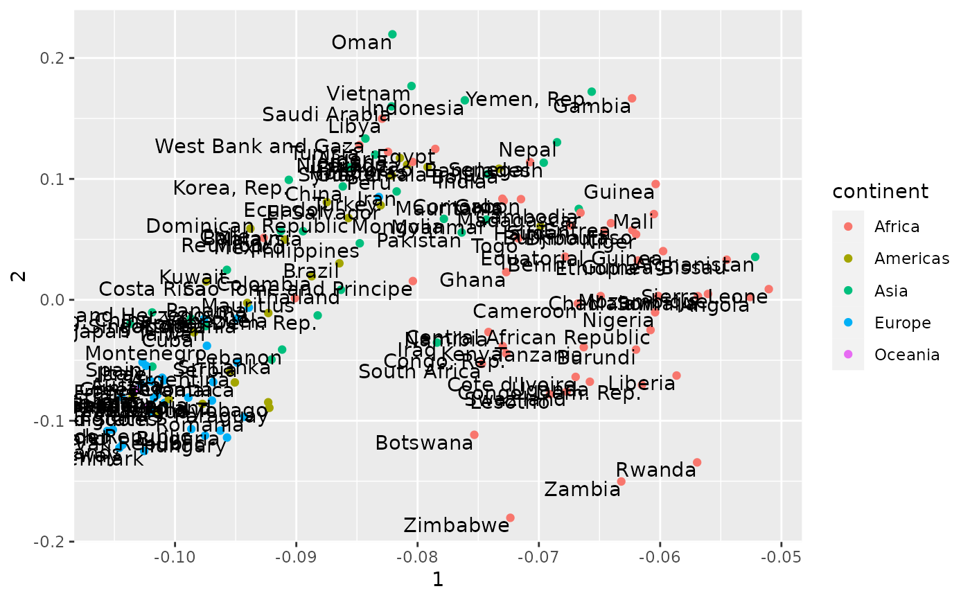
gapminder_svd %>%
  spread(dimension, value) %>%
  inner_join(distinct(gapminder, country, continent), by = "country") %>%
  ggplot(aes(`1`, `2`, label = country)) +
  geom_point(aes(color = continent)) +
  geom_text(vjust = 1, hjust = 1)